engiAI
- Requirements
- What it does
- Licensing
The engiAI interface is available in English: button and field names in this manual are given exactly as they appear in the program.
Contents
- 1. Why engiAI and the ZONE-PAIR method?
- 1.1. What advantages does this method offer compared to classifying the entire frame?
- 1.2. Speed: The AI only focuses on the relevant excerpts.
- 1.3. What level of accuracy can be expected: calculating based on our camera
- 1.4. Quick Start: Settings are pre-configured, and the zones and model can be set up in just a few clicks.
- 2. Learn the program interface in one minute
- 3. Cameras: Connection and Setup
- 3.1. Which cameras are supported?
- 3.2. Camera Window: Add, Reconfigure, or Remove
- 3.3. Camera tab for HIKROBOT and SICK
- 3.4. Camera Tab for USB/Webcam
- 3.5. Saved Camera Settings (Presets)
- 3.6. GigE Network and Reconnection
- 4. The ZONE-PAIR Model: From Grid to Trained Model
- 4.1. How the method works: one model, one class per zone
- 4.2. Develop a model
- 4.3. Mark payment areas
- 4.4. Record the reference: alignment region
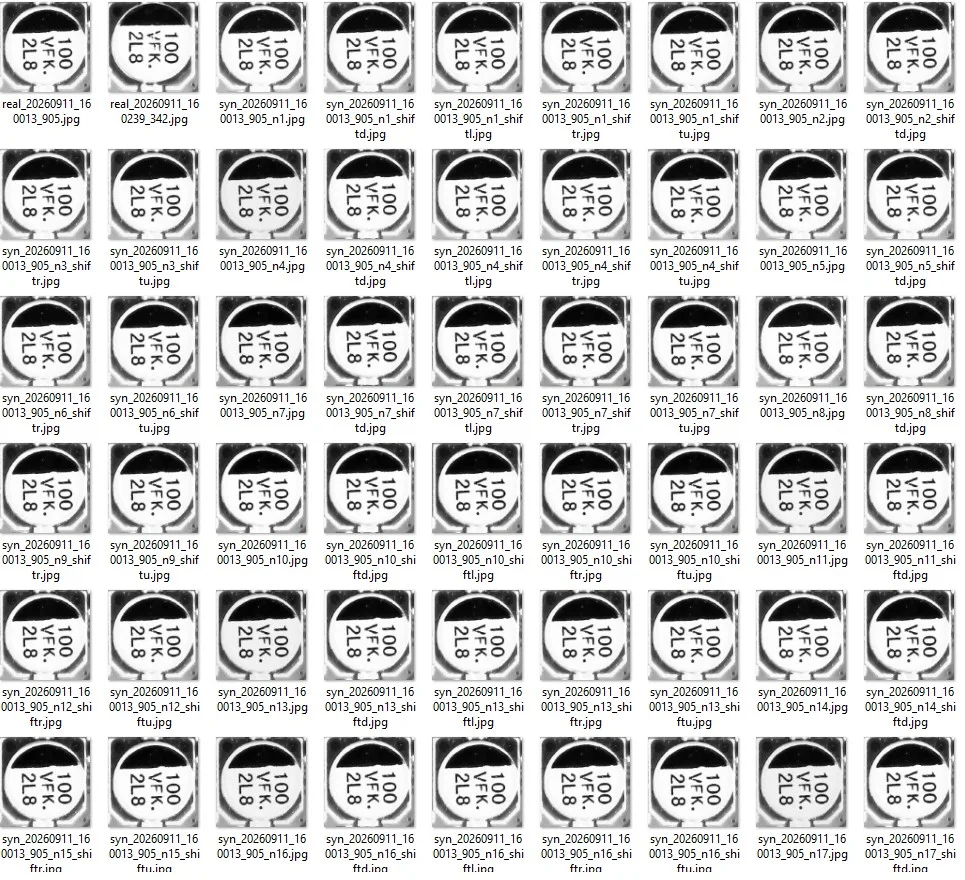
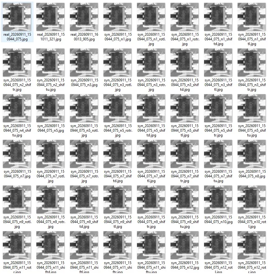
- 4.5. Zone-based image: normal and its synthetic data
- 4.6. Synthetic data defect: The element shifts along with the base with just two clicks.
- 4.7. Anomalies in Zones: Settings Window
- 4.8. References to zones: solder pads and zone editor
- 4.9. Model Training
- 5. Inspection
- 5.1. Assign a model and verify the zones.
- 5.2. Zone Recognition Threshold
- 5.3. The "Live Conveyor": Payment in Any Position
- 5.4. Which signal should be analyzed?
- 5.5. Yellow Zones: Turn off the zone by clicking
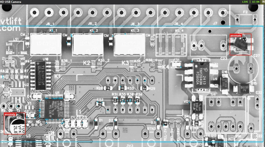
- 5.6. What you can see on the screen and in the console
- 6. Triggers: External sensor on the camera's input
- 7. Outputs: rejector, discrete outputs for cameras, and TCP
- 7.1. Reference: Outputs: Contacts and Tester Verification
- 7.2. OUTPUT Window: Rule for the Zone
- 7.3. Sending a TCP packet to the robot or PLC
- 7.4. Discrete camera output
- 7.5. Audio alerts: a unique sound for each zone
- 7.6. Log of activations and database
- 8. Other modes and tasks
- 9. Settings, console, requirements, and license
- 10. A concise checklist and troubleshooting guide
How to use the manual: Section 1 explains the purpose of the method and the expected results. Sections 3-5 outline the steps from a blank program to a working inspection, and should be followed in order. Sections 6-7 cover sensor, output, and TCP connections. Sections 8-10 cover the remaining features, settings, and a checklist.
1. Why engiAI and the ZONE-PAIR method?
engiAI Ethernet System – a visual inspection program for production lines. It takes a frame from an industrial or standard camera, divides it into zones, checks each zone using a trained neural network, and converts the result into an action: a signal to the camera's discrete output, a TCP message to a robot or PLC, or a record in a log. The ZONE-PAIR method is designed for products where each location has its "correct" component: printed circuit boards, assemblies, sets of parts in a tray, and packaging with specific layouts.
1.1. What does the method offer compared to classifying the entire frame?
A common approach is to use a single model with two classes, "normal/anomaly," applied to the entire image or to specific zones. However, this doesn't work on the circuit board: a gap under the BR1 bridge in zone 2 indicates a defect, while the same gap in another area of the board is considered normal. A single model cannot distinguish between these two cases. The other extreme is to use a separate model for each component, which would require dozens of training runs and numerous files in memory.
ZONE-PAIR addresses this by using a single model, with as many classes as there are zones. A "Zone" is a rectangle surrounding a single component. A "Class" is a folder containing images that the network learns from. Each zone has its own pair: "zone_001" (normal zone 1, for example, the C30 capacitor) and "zone_001_anomaly" (defect zone 1); "zone_002" and "zone_002_anomaly" represent the BR1 bridge. When checking zone 1, the program only looks at its pair; the answers for zone 2 are not used. Anomaly classes are optional: the "defect" changes the appearance of the zone, and the confidence in the "normal" state decreases automatically; however, with synthetic data (section 4.6), they can be created with a single click and noticeably improve reliability.
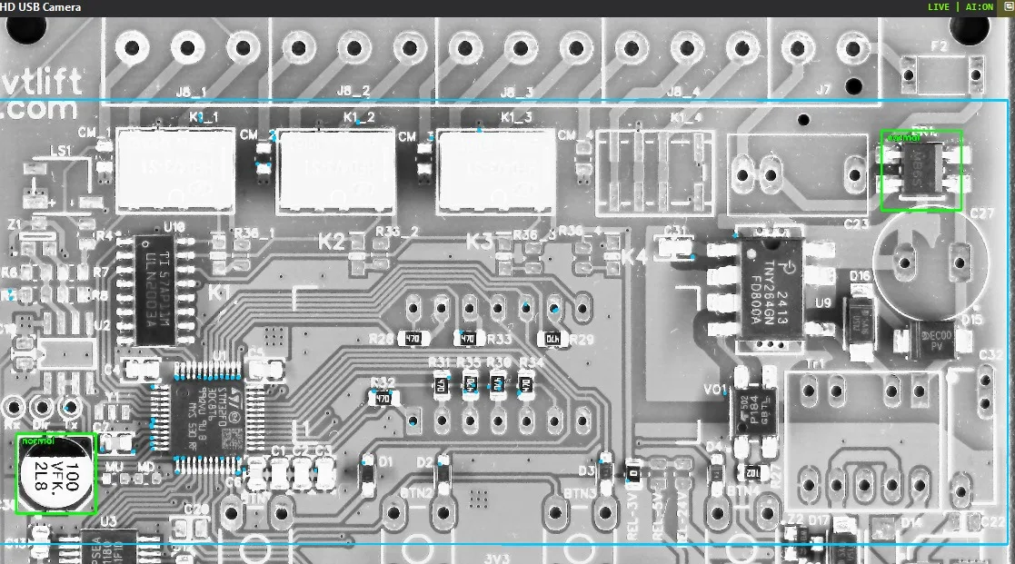
1.2. Speed: The AI only looks at the relevant sections
The neural network never receives the entire frame. Only the rectangle corresponding to each zone is extracted, and the zone number is selected from two classes. Zones from a single frame are processed in parallel (up to four threads), and the results from all zones are displayed together as a single batch, rather than one zone at a time.
- The analysis speed is determined by time. The "Analyses per second (AI)" slider on the Camera tab indicates exactly N analyses per second, not "every Nth frame." The limit is the camera's frame rate and inference time.
- GPU is used by default. Inference is performed using ONNX Runtime with CUDA; if there is no NVIDIA graphics card, the program automatically switches to the CPU and indicates this in the status (GPU (CUDA) or CPU).
- Clean buffers. Memory allocated for clippings is used once per stream and then reused; analysis time remains consistent across frames.
- Model for the task. For ZONE-PAIR, the program automatically sets the input size to 128 px and uses the YOLO11 "s" size network: the extracted zone is barely scaled, and the network has sufficient capacity to handle hundreds of pairs of classes.
- A live conveyor saves labor. The operator doesn't need to manually move the parts through the process as frequently as in a traditional system; the parts are picked and aligned once, and then the cutting is performed.
- The display does not interfere with analysis. The tile is redrawn no more than 25 times per second, and only based on the new frame from the camera. The image is reduced to the size of the tile before being displayed on the screen, and the log is written to a file by a background thread. The interface remains responsive even with 8-megapixel frames and hundreds of zones.
Displayed above the video, in the status bar, are the actual figures: fps (frames per second) and the milliseconds of the last analysis, as well as Eff, which indicates how many analyses were actually completed per second.
1.3. What accuracy to expect: Let's calculate using our camera
The program does not guarantee a "0.5 mm" shift regardless of the camera and lens. The sensitivity to displacement is determined by how many pixels correspond to one millimeter of the object, and by the boundary that the model has been trained on. This is calculated in two lines:
Minimum perceptible shift ≈ 5 px ÷ (px/mm)
The number 5 px represents the lower limit of the synthetic shift in the recommended settings for anomalies (with a standard deviation of 0–2 px). The default settings are based on 11 px/mm: at this scale, 0.5 mm corresponds to 5–6 px, which is the target value that was agreed upon during development. Please enter your own values:
| Camera (frame width) | Field of view 100 mm | 200 mm | 300 mm | 400 mm |
|---|---|---|---|---|
| 3264 px (USB 8 MP, as in the images) | 0.03 mm/px → shift ≈ 0.15 mm | 0.06 → ≈ 0.3 mm | 0.09 → ≈ 0.45 mm | 0.12 → ≈ 0.6 mm |
| 2448 px (HIKROBOT 5 MP) | 0.04 → ≈ 0.2 mm | 0.08 → ≈ 0.4 mm | 0.12 → ≈ 0.6 mm | 0.16 → ≈ 0.8 mm |
| 1920 px (SICK picoCam, HIKROBOT 2 MP) | 0.05 → ≈ 0.25 mm | 0.10 → ≈ 0.5 mm | 0.16 → ≈ 0.8 mm | 0.21 → ≈ 1.0 mm |
1.4. Quick Start: Settings pre-configured, zones and model ready in a few clicks
This method is designed to allow a technician with no prior experience in machine learning to obtain a working model in a single shift. Everything that could be pre-configured is already configured and stored in the program's database:
- Zones per minute. In the ROI editor, drag a frame around the element and specify the zone size (e.g., 256 px). If there are many elements arranged in a grid, drag the frame across the entire layout – the program will automatically calculate the rows and columns of the grid.
- Synthetic data for normal and defective scenarios is pre-configured. The "Default," "Element Offset," and "Color and Texture" buttons switch between pre-defined profiles. The number of files, camera frames, and expected time are displayed before the "Capture" button is pressed.
- The training parameters are set automatically. After the initial scan, the program sets the Image Size to 128, Model Size to s, Epochs to 50, and Batch to 64, and disables augmentations during training that conflict with the anomaly classes.
- The camera is adjusted using a button. The "Auto-setting for AI (per frame)" function automatically selects the shutter speed, amplification, gamma, and white balance; for USB cameras, there are "Auto-selection for forms" and "Set parameters" options.
- Camera settings packs. The selected settings are saved under a specific name and can be switched between from a list. The camera immediately accepts and stores these settings in its memory.
- One ONNX file as output. The trained model is automatically exported and immediately assigned for inspection; no further steps are required.
The entire process: connect the camera → create a model → mark zones → define the alignment region → take "Zone Images" on multiple functional boards → identify "Zone Anomalies" → TRAIN AI MODEL → Inspect tab. The remaining steps involve assigning sound, outputs, and TCP connections to the zones. To get started, you will need a computer with Windows 10/11 (a NVIDIA graphics card is recommended for faster inspection), a camera, one functional board, and one internet connection for installing the training environment. Defective boards are not required.
2. Program Interface in One Minute
The main window is divided into two parts. On the left is a live video feed from the cameras and a status bar above it. On the right is a panel with tabs, where all the controls are located. The user can drag the boundary between the two sections; the program remembers the size, position, and layout of all windows in its database.
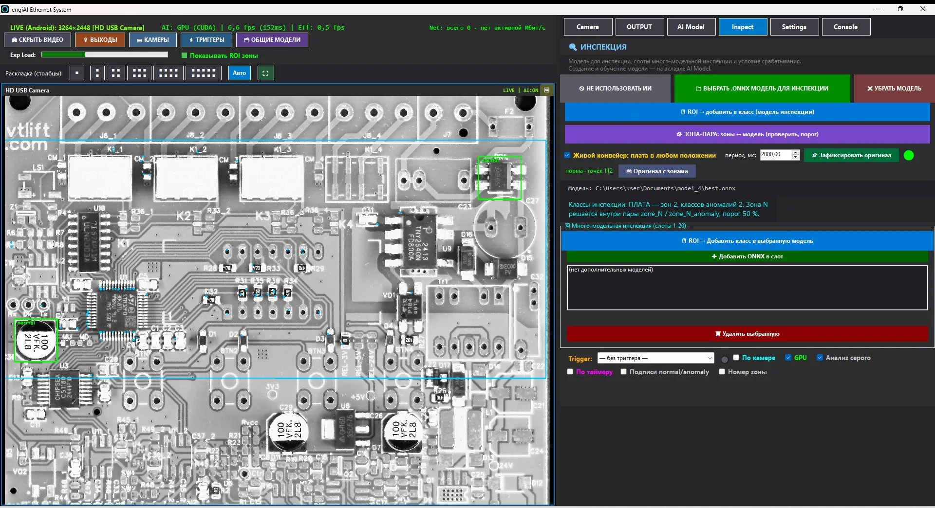
Buttons above the video
| Button | What it opens |
|---|---|
| HIDE VIDEO | Removes the image from the screen. Analysis continues, only rendering is saved. |
| OUTPUTS | Reference window: contact information for discrete camera outputs from HIKROBOT and SICK, testing, connecting a load (section 7.1). |
| CAMERAS | "Camera Settings" window: adding, reconnecting, and deleting cameras, and viewing all parameters read from the hardware (section 3.2). |
| TRIGGERS | Connecting an external sensor to the camera's discrete input with a diagram and pinout (section 6). |
| GENERAL MODELS | Named sets "camera → model", assigned to the entire stand with a single selection (Section 8). |
| Layout (columns) | How many camera tiles to display in a row; "■" - single mode (selected camera zoomed in), "Auto" - based on the number of cameras, "⛶" - cameras across the entire monitor (Esc key). |
| Display ROI zones | Draw a grid of zones on the video. |
Tabs on the right
| Tab | Purpose |
|---|---|
| Camera | Parameters of the selected camera: shutter speed, amplification, color, resolution, automatic settings for AI, saved settings, analysis speed. The AI threshold is no longer available here - it is only on the "Inspect" tab. |
| OUTPUT | rejector: rules on zones - TCP packets to the robot/PLC, discrete camera outputs and audio alerts, event log, database. |
| AI Model | Creating a model: folder, classes, zone grid, zone snapshots, zone anomalies, reference boards, settings and training start. |
| Inspect | Working tab: which model is inspecting, inspection zones and threshold, live conveyor, which signal to capture, multi-model inspection slots. |
| Settings | Interface language (14 languages), license purchase, saving and loading settings, video recording. |
| Console | Event log: camera connection, training progress, rejector activation, warnings. The screen displays the 800-1000 most recent lines, and all data is written to the files logs\engiai-*.log. |
Status bar
The status of the active camera is displayed above the buttons: `LIVE (Android): 3264×2448 [HD USB Camera] – type, resolution, and name; `AI: WAITING or `AI: GPU (CUDA) – the model's assessment and the number of milliseconds taken for the last analysis; `Net: total … active … Mbit/s – network load from GigE cameras (green up to 40% of the link, orange up to 70%, and red thereafter). The `Exp Load bar shows what proportion of the frame interval is occupied by the exposure time: if it reaches the right edge, the camera will not maintain the specified frame rate.
Each camera's tile displays a header with the camera's name, status (LIVE | AI:ON), and a reconnect button. Right-clicking on a frame opens the zone menu, while right-clicking and dragging allows you to pan across the zoomed-in frame.
3. Cameras: connection and configuration
3.1. Supported cameras
| Type | How to connect | What can be configured from the program |
|---|---|---|
| HIKROBOT MV-CS (GigE, USB3) | Native MVS SDK. Opens strictly by serial number, the order of listing is irrelevant. | Exposure time: 6 μs, gain in dB, FPS, resolution (AOI), black level: 0…4095, all GenICam nodes (auto modes, gamma, sharpness, white balance R/G/B, digital shift, flip, GigE packets). Parameters are written in the UserSet1 of the camera itself. Discrete input Line 0, output Line 1, GPIO Line 2. |
| SICK picoCam (IDS uEye, GigE) | uEye driver. The camera should be visible in IDS Camera Manager with the status "configured correctly". The serial number is verified with the camera because the DeviceID in uEye changes with each start. | Gain, amplification 0…100, FPS, resolution, black level 0…255, pixel clock, gain boost, hardware amplification of channels R/G/B, hardware gamma, Bayer pattern. Parameters are written to the camera's memory. Trigger input on the optocoupler, Flash output (150 mA). |
| USB webcam (in the list - Android) | DirectShow via OpenCV, differ in moniker, so two identical cameras do not get confused. | Up to 8K resolution, FPS, all driver properties: brightness, contrast, saturation, hue, sharpness, gamma, amplification, shutter (auto), focus (auto), white balance (auto), backlighting compensation, etc. There are no discrete inputs and outputs; only TCP is available. |
| IP Camera RTSP | The link in the format `rtsp://admin:password@192.168.1.64:554/…` must be entered manually. | Shutter, amplification, resolution, and FPS are set in the camera's web interface. The program includes zones, model, and TCP. |
There is no hard limit on the number of cameras: tiles can be arranged in a grid with any number; eight and nine cameras worked simultaneously on real setups. Each camera has its own model, its own zones, its own threshold, and its own analysis speed.
3.2. CAMERA WINDOW: Add, reconnect, delete
The checkboxes below apply to the selected camera: Camera enabled (otherwise, it will be disconnected from the device and disappear from the screen), Show video/zones (this only controls the display; analysis always runs), AI enabled for the selected camera. The Reconnect button performs a complete disconnection and reconnection, restarting the AI stream and reloading the models.
The right-hand side of the window displays all the camera parameters read from the hardware upon connection, grouped and with units of measurement: "Show parameters for," Re-read from camera, Copy to clipboard. This is only for viewing; you can change the parameters on the "Camera" tab.
3.3. Camera Tab for HIKROBOT and SICK
The tab controls the camera, with the camera tile highlighted by a blue border. When the program is connected, it does not write any data to the camera; instead, the camera serves as the source of truth, and the sliders adjust to match its values. Settings can only be saved intentionally by pressing the "Save settings" button.
"Hikrobot: Camera Parameters (GenICam)" block
Only the data captured by the camera is displayed. The following settings are available: Auto Exposure (Off / Once / Continuous), Auto Gain, Gamma and Gamma Mode, Sharpness, Hue, Saturation, Auto White Balance, White Balance by Channel, Digital Shift, Black Level Enabled, FPS Limit Enabled, Horizontal and Vertical Flip, GigE: Packet Size, GigE: Inter-Packet Delay, GigE: Bandwidth Limit, Test Image. The "Read Parameters from Camera" button updates the table.
"IMAGE COLOR" block
Bayer pattern (Auto / BGGR / RGGB / GRBG / GBRG), Saturation 0…200 %, Gamma 0.30…3.00, Contrast 50…200 %, reset button. Software processing is applied to all frame consumers: display, recording, inference, and training images, so the image is the same during training and inspection. For HIKROBOT, the pattern is taken from the camera pixel format, while for color SICK sensors, it is taken from the sensor and refined based on the first frame.
| Parameter | What it does | What it affects |
|---|---|---|
| Analysis per second (AI) | Upper limit of inspection speed: 1…200 | Lower values result in lower strain on the graphics card; independent of camera connection. |
| AI threshold: | Not set on the "Camera" tab. | Zone recognition threshold: only on the "Inspect" tab (section 5.2), one per camera. |
| Exposure | Exposure time: | Shorter exposure times result in less blurring of moving objects; a value of zero is not allowed. |
| Gain / Gain boost | Matrix signal amplification: | Increases brightness, but also adds noise. |
| Pixel clock (SICK) | Sensor clock frequency: | Changes the FPS and exposure ranges, which are re-read. |
| FPS | Frame rate in free mode | Not used in trigger mode |
| Width / Height | Frame size (AOI) | Smaller frame = higher frequency and less traffic |
3.4. Camera Tab for USB/Webcam
For USB cameras, the tab displays the "USB Camera: Resolution, FPS, and Properties" block. Properties of the driver that the camera does not provide are not displayed; the field boundaries are set by the program because DirectShow does not report ranges.
3.5. Saved Camera Settings (Sets)
The "Saved Camera Settings" block is displayed for USB, SICK, and HIKROBOT cameras. By selecting the parameters for the product, save them under a name: for another board or different lighting, simply select a set from the list.
- Save as… – Reads the current values from the camera and prompts for a set name. If the name is already in use, it offers to overwrite it.
- Selecting a set from the list immediately writes the parameters to the camera and saves them: for USB, to the database; for SICK and HIKROBOT, to a parameter file and the camera's memory (UserSet1 / EEPROM). Then, the panel reads the values from the hardware and displays how many parameters have been accepted and how many have been deviated from.
- Overwrite overwrites the selected set with the current values, Rename and Delete only affect the database entry; the camera settings remain unchanged.
The kit includes: for USB – resolution, FPS, driver properties, and auto-modes; for SICK – gain, exposure, FPS, black level, pixel clock, gain boost, white balance R/G/B, hardware gamma, and software color; for HIKROBOT – gain, exposure, FPS, black level, and all GenICam nodes. The frame size of industrial cameras is not included in the kit; changing it restarts the capture. The kits are the same for all cameras of the same type, so one kit is placed on each camera on the stand.
3.6. GigE Network and Reconnection
- The HIKROBOT GigE packet size is automatically set to optimal when opened; it can also be manually adjusted in the GenICam block. Jumbo frames (8164–9000) reduce the load; when using fragmented frames, set 1500 and increase the inter-packet delay.
- The `Net` line calculates the load from each camera based on its own data (useful load × frequency) and compares it to the actual incoming network traffic. A significant discrepancy indicates dropped frames or extraneous traffic. Virtual adapters and NDIS filters (GigEVision, uEye, Npcap) are excluded from the calculation.
- If the camera is visible but the stream isn't working, click "Reconnect" (in the CAMERA window or on the tile). The most common causes are network bandwidth limitations or USB bandwidth issues.
- The SICK picoCam loses its settings when the descriptor is closed; if there is no configuration file in the camera itself, the program applies the configuration file and prompts the user to click "Save Settings" to save them to the camera.
4. ZONE-PAIR Model: From Grid to Trained Model
4.1. How the method works: One model, one class per zone
The ZONE-PAIR model is a standard YOLO11 classification network, with a number of classes equal to the number of zones, plus optional anomaly classes. A class consists of a folder within the `train` and `val` directories. The program automatically creates all folders; no manual creation is required. Here is an example of a model's folder structure after training:
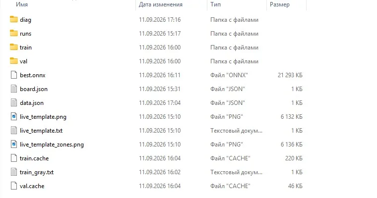
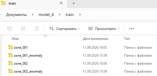
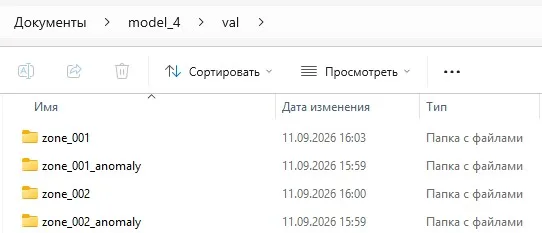
The files named `real_…jpg` are actual images captured by the camera (and are included in both the training and validation sets). The files named `syn_…jpg` represent synthetic data. The files named `edit_…jpg` are images taken from the zone editor. In the example provided, after capturing images of several boards: `zone_001` contains 502 files in the training set and 111 in the validation set; `zone_001_anomaly` contains 680 files in the training set and 144 in the validation set; `zone_002` contains 813 files in the training set and 181 in the validation set; `zone_002_anomaly` contains 340 files in the training set and 60 in the validation set.
The program automatically recognizes the model as a "payment" based on the presence of the zone_NNN class. The class number is the zone number within the grid (1…N). Therefore, the main rule of the method is:
4.2. Create the model
4.3. Mark zones on the board
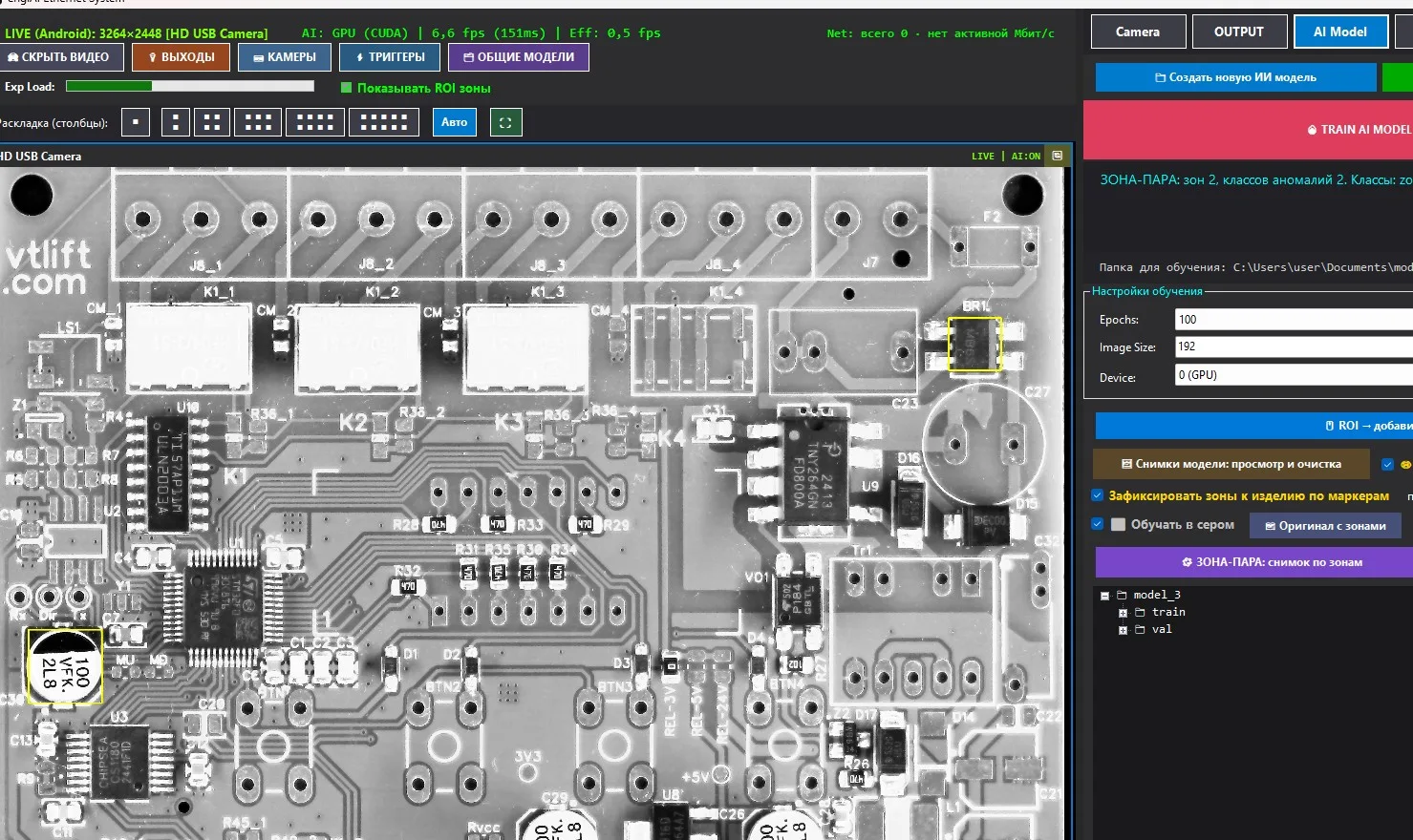
Red zones: Exclude a zone from synthetic data with a single click
On the "AI Model" tab, click on the already created area directly on the video with the left mouse button: the area will turn red and will no longer be part of the zone-based and anomaly detection. A second click will restore it. The file counters in the synthetic data windows are recalculated immediately, and the "off N" label above the frame indicates how many areas are turned off. The list of red areas is stored per camera and model; on the "Inspect" tab, the same area remains normal (with its own yellow areas – section 5.5).
4.4. Fix reference: alignment region
The inspection zones are defined based on the position of a single circuit board. To allow for the insertion of another board with a shift and rotation, the software remembers a reference point: a live frame and an alignment region – a section of the board with features that are used to locate the product in each new frame. Once the area is found, the software transfers the inspection zones to the new board. This is how the image acquisition, synthetic data generation, and inspection processes work.
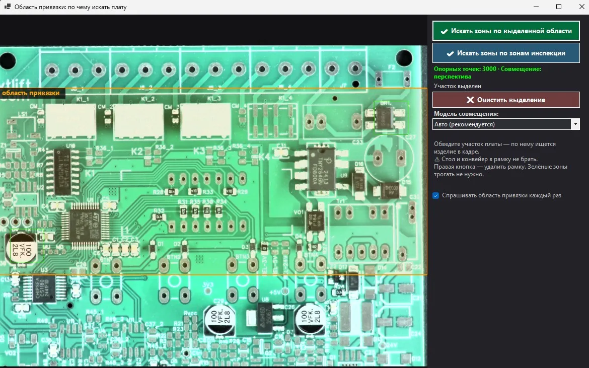
| Alignment model | When to use |
|---|---|
| Automatic (recommended) | The board is aligned rigidly (translation, rotation, scale); the perspective is only connected if it aligns significantly better. Accuracy in a small alignment region – 1–2 px. |
| Rigid | The camera looks straight down, the board lies flat. The most stable option if the alignment region is small. |
| Perspective | The camera is at an angle or the board is tilted. A large area with points across the entire width is needed, otherwise the homography will "skew". |
The "reference with zones" button opens the saved reference with a grid and zone numbers (section 4.8). The found component is checked for reasonableness: the area should be between 0.5 and 2 times the area of the reference, it should be a convex quadrilateral, and the support points should occupy at least a quarter of the area along each axis – otherwise, the result is discarded, and the message "component not found" is displayed in the console.
4.5. Zone-based image: normal and its synthetic data
The "ZONE-PAIR" button: creating a zone-based image involves cutting the live image into zones, placing each zone's excerpt into its corresponding class zone_NNN, and adding synthetic data representing normal conditions. Synthetic data representing normal conditions is not a defect; it reflects variations in the image, such as a slightly different placement of the board, slightly different lighting, and sensor noise.
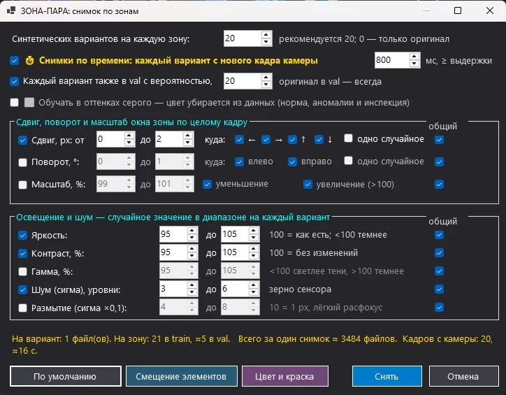
| Settings | What to create and default settings |
|---|---|
| Synthetic options for each area | How many synthetic files to create per cutout. Recommended: 20, 0 (only reference), maximum 500. |
| Time-stamped images: each option from a new frame from the camera | Enabled, period 800–1200 ms (at least the exposure time). Each option is taken from a new live frame: real sensor noise, vibration, and light flicker instead of being drawn. |
| Each option also in val with a probability of % | 20% reference always appears in val: Ultralytics requires each class to be in both folders. |
| Train in grayscale | Overall model flag: color is removed from normal, anomalies, and inspection. It is not possible to mix color and grayscale files in one model; the program will warn you. |
| Shift, px · to where | The sliding area shifts across the entire frame by 0…2 px in the specified directions (← → ↑ ↓); the missing strip is taken from the adjacent area on the circuit board, and the cutout remains even. The checkbox all directions provides a separate file for each direction, while one random provides a single file. |
| Rotation, ° · to where | By default, it is disabled: no rotation is applied to the alignment region, and enabling it blurs the boundary with the defect. The options "left/right" and "all directions/random" function similarly to the shift option. |
| Scale, % · decrease/increase | By default, it is turned off. Two checkmarks represent two sides: reduction (<100) and increase (>100, the zone window takes neighboring frames). Each marked side corresponds to a separate file. |
| Brightness/Contrast/Gamma | Random value from the range for each option: brightness 88…112, contrast 88…112 %, gamma 98…102 % (in the image); in the "Element Offset" profile, the brightness is wider to avoid being mistaken for a defect. |
| Noise (sigma) / Blur | Sensor grain 3…8 levels, slight defocus 0.4…0.8 px. |
| "General" column | With the checkbox, the view is included in the general file along with the others; without it, a separate "reference + only this view" file is created. The more individual views, the more files are created per option. |
4.6. Synthetic data defect: element shifts with the base
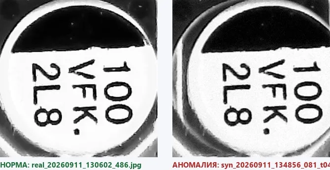
The synthetic data is based on observation. The model learns particularly well when, instead of a drawn-out stain, it is presented with the inspected element itself, along with the surrounding components of the circuit board: including silk screen lines, tracks, color, and the texture of the base. The program reduces the frame to the size of the element and then shifts or rotates this area, filling the edge with adjacent pixels from the frame. As a result, the element is not in its original position relative to the base: exactly as the inspector would see it in a real defect, with real sensor noise, real lighting, and a real circuit board.
The "normal" and "anomaly" zones within a region differ only in the position of the element relative to the base. Everything else is the same, so the network learns the relationship "element ↔ board," rather than the shade of a spot or the lighting.
Two clicks:
No further configuration is required: you don't need to draw defects or search for faulty boards. Next, TRAIN AI MODEL.
Before and after: what the program achieves
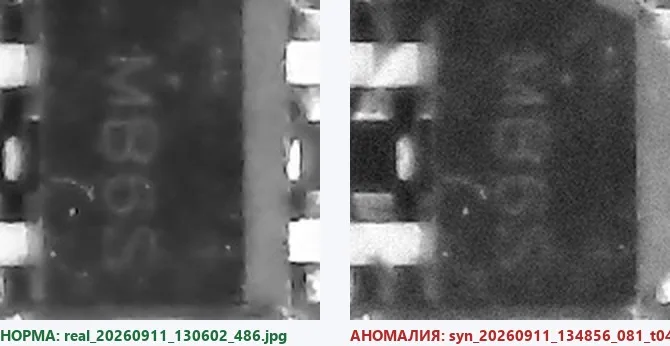
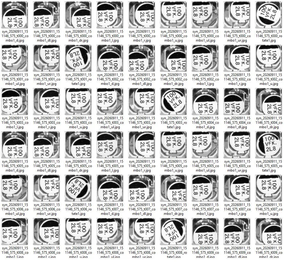
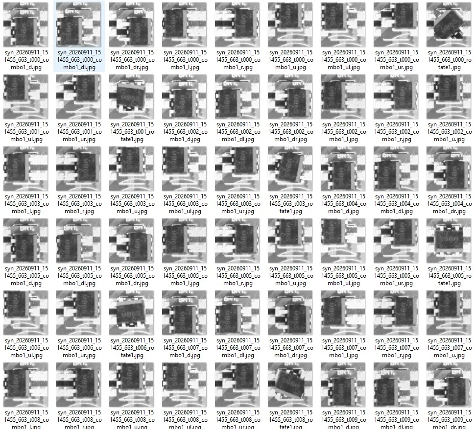
Folders representing anomalies as seen by the user
Compare with the "normal" folders from section 4.5: the only difference is the position of the detail relative to the base.
Detail marking: why is the "thick" line and how is it configured?
The parts have markings – labels and 1–2 px thick lines within the frame. These markings vary from batch to batch: different fonts, labels on capacitors are rotated, and some symbols are erased. If a synthetic defect, such as a "scratch," is drawn with the same thin line, the system will not be able to distinguish it from the marking line and sensor noise, and will begin to reject boards from a different batch.
The synthetic data ZONE-PAIR addresses this from both sides. First, the main defect – the displacement of the element – moves the marking along with the body, so the marking does not become a distinguishing feature: it looks the same in both normal and anomalous states. Second, the default line/scratch is thick (⅛ of the zone, no less than 3 px) and is clearly not a marking stroke. The thickness is now explicitly defined: the Line thickness, px (0 = auto) field applies to both the line and the cross.
Hand-drawn defects (rectangles, circles, lines, "missing element," blurred spots, and others) are grouped together in a collapsible section Synthetic defects on top of the cutout. By default, it is collapsed and disabled: the main defect on the board is misalignment. Enable it for specific tasks: flooded area, extra drop, worn-off marking.
| Figure parameters | What it defines |
|---|---|
| Size: from … to, % of the zone / px | The size or length of the figure. In percentages, it is proportional to the smaller side of the zone; in px, it is the same for all zones, which is convenient when the actual defect size in pixels of the frame is known. |
| Fill | solid / outline / mixed (outline is also thick). |
| Line thickness, px | Line / scratch and cross. 0 — auto (thick). For marking details, do not go below 3 px. |
| Where the defect is | Center, left, right, top, bottom – where to place the piece (with a slight random variation). Checkmark all provisions - a file for each marked location; A random occurrence - One file is selected randomly from the marked files. The file counter at the bottom of the window automatically reflects this selection. |
| Figure colors: 5 slots | Five slots instead of a list of names. A checkmark indicates that the slot is active, and the color is randomly selected from the marked options (±12 per channel, to avoid a single shade). The "sample" button allows you to choose a color from the palette, while the "dropper" (represented by 💧) allows you to click on a live camera frame (the wheel controls zoom, and the right button controls panning) to select a color from a real object or component. Two slots are enabled by default: one for dark and one for light colors, while the other three are disabled. |
| "General" column | The marked defect type is placed in the general file along with other "common" types (e.g., a scratch on an element that has been shifted). Without the checkbox, the file will contain "normal + only this defect". The "all positions" view will always be in a separate file. |
4.7. Zone Anomalies: Settings Window
The `ZONE-PAIR` button: "Anomaly Zones" creates classes `zone_NNN_anomaly` from normal cuts. All zones are selected, except for the red (disabled) zones (created by clicking on the AI Model frame in section 4.3). Anomaly classes are not needed everywhere: add them to zones where defects actually occur, and the model will check the remaining zones for recognition.
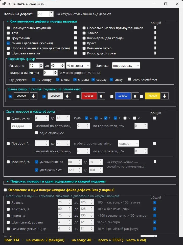
| Settings | What it does |
|---|---|
| Copies the defect | One number for all types: how many copies with new random parameters to create for each marked type (default: 10). |
| ▸ Synthetic defects on the cutout | Default group: rectangle, small rectangles, circle, ellipse, triangle, octagon, line/scratch, cross, `missing element`, blurred spot, noise patch, piece from another area. Figure parameters, location, and palette – Section 4.6. |
| Shift, px · where · shape | Main defect of the board. The area (circle or square) shifts by 5–12 px in the specified directions: ← → ↑ ↓ and the two diagonals ⤡ ⤢. scale vertically / horizontally, ±% – the size of the area relative to the zone: 0 – the entire zone, -30 – an area 30% smaller (only the element shifts, the base remains), +30 – an area larger than the zone (captures neighboring elements from the frame). all directions – for each side, according to the file. |
| Rotation, ° · shape | The area (circle or square, same scale ±%) rotates to a random angle in both directions. |
| Scale, % · decrease/increase | The area as a defect: reduction of 60–85% or increase of 120–160%. Each marked side is its own file. Usually disabled on the board. |
| "General" for shift and rotation | If both checkboxes are selected, it means one element in one file: the translation and rotation are applied through a single transformation (not sequentially, otherwise it would result in a "mess"), the area scale and shape are common and defined by the translation. |
| ▸ Sub-zones | The area is divided into 2, 4, or 9 parts, and within each, a separate area rotates or shifts; the "separate photo for each sub-zone" option creates a file for each part. This is needed for large areas with multiple elements. |
| Lighting and noise on each defect file | Enabled and set to normal: the defect should differ in geometry, not in lighting. |
| Photos over time / in val | Each copy from the new camera frame (800 ms), 20% in val, the first file in the val class is always present. |
4.8. Reference with zones: solder pads and zone editor
The "reference with zones" button opens a saved reference image with a grid. Synthetic data is created here without a camera: the zoom function, the right button for panorama, and the left button for selecting zones (Ctrl to add, drag with the mouse to define the area, Ctrl+A to select all), and double-clicking opens the zone editor.
- Solder pads for selected areas… – "Solder pads: short circuit between tracks". The program automatically identifies tracks within the area (Ozu threshold, light-colored strips ≥ 2 px), placing a solder pad in the gap between adjacent tracks, using the color of the tracks, with a dark border and a highlight. Settings: between vertical or horizontal tracks, pads for images 1…3, size 8…18% of the area, images per area (5), where to place – in an anomaly or in normal, surface lighting, in val – a new image with different lighting or an exact copy.
- Zone Editor: Tools: Brush, Pipette, Color Spot, Copy Area, Paste, Stamp, Area for pads; palette: "solder / pad", "board", "shadow / mask", white, black; "Copy" field and Create Image button. This allows you to draw a defect that was not present on the line: a filled pad, an extra element, or a missing label.
The editor's files are named edit_… and are categorized into either the "zone" class or its "anomaly" class. On the "Inspect" tab, the same window opens, but it is only for viewing purposes.
4.9. Model training
The "Training Settings" section on the AI Model tab is automatically populated after the initial scan based on the specified zones: Image Size 128, Model Size s, Epochs 50, Batch 64. These values correspond to the 108–137 px zones. For the 256 px zones, as in the example, set Image Size to 192 or 256 – this will minimize compression (the Epochs 100 and Image Size 192 settings are shown in the main window). Verify the values and click "TRAIN AI MODEL".
| Parameter | What it means | How to choose |
|---|---|---|
| Epochs | How many times the model will process the entire dataset | 50 for the default board; 100-150 if there are many anomaly classes |
| Batch Size | How many images per step | 64; reduce if there is insufficient video memory |
| Image Size | What size are the crops, divisible by 32 | Approximate zone size: 128 for a 108-137 px zone; 192-256 for 256 px zones, as in the example |
| Model Size | n / s / m / l / x | s — optimal for hundreds of pairs of classes; n is insufficient capacity, m and above — slower |
| Device | On what to train | 0 (GPU) with an NVIDIA graphics card; without CUDA, the program will automatically switch to the CPU |
| Workers | Number of data preparation threads | 12 (default for a multi-core processor) |
5. Inspection
All the work is done on the "Inspect" tab. The model has already been trained; now it's necessary to check the regions, set the threshold, select the speed source, and, if the board arrives in any orientation, enable the "live conveyor" feature.
5.1. Assign the model and check the zones
5.2. Zone recognition threshold
For each zone, the network provides probabilities for all classes, but the decision is made only within each pair. The probability of the "normal" class, q, is calculated as p(zone_N) / (p(zone_N) + p(zone_N_anomaly)) and is then multiplied by a "confidence" factor, which represents how likely the pair is to be considered a valid output by the network (full confidence is achieved at 10% or higher). The resulting score, ranging from 0 to 100%, is compared to a threshold: a score above the threshold indicates a "normal" state, while a score below the threshold indicates an anomaly.
The default threshold is 50%, and it is stored in `board.json` alongside the model and applied immediately without requiring a restart. Below 50%, the threshold shifts towards normal more strongly: 25% → a cutoff of 6%, 10% → 0.4%, 1% → almost all green; 99% only allows through confident areas. This scale is needed so that the operator can distinguish between 5% and 99%, rather than seeing only areas in red.
5.3. Live pipeline: payment in any position
Halo Live Conveyor: Finding the PCB in Any Position includes searching for the PCB based on its alignment region before each analysis: the frame is aligned with the reference image, the cutting zones are extracted from the aligned image, and the alignment region and zones (green – normal, red – anomaly) are drawn on the video. The field Period, ms specifies how often to search for the PCB (default: 1000, 2000 in the image). The indicator next to it indicates: "normal · N points", "ANOMALY · N points", or "PCB not found" or "No reference – confirm". The verdict is based on a single analysis, without accumulation.
The reference and alignment region are fixed using the same button Fix reference, as when taking a picture (section 4.4); reference with zones opens it for viewing. The boundaries of the alignment region and the blue reference points, which align the board, are drawn on the video. Areas that extend beyond the frame after alignment are marked with the SKIP label.
5.4. Analyze based on which signal
The source of the speed is always the same: when a new one is included, the program removes the previous one.
| Method | How to enable | When to use |
|---|---|---|
| By camera | "By camera" checkbox | Continuous monitoring; speed limited by the "Analyzes per second" slider on the Camera tab |
| By timer | "By timer" checkbox and interval (ms) | Periodic monitoring, for example, once per second |
| By trigger | Select a connection from the "Trigger" list and a front ("analyze + on input" or "analyze -") | Camera-based conveyor: a frame is captured at the moment the product arrives – the most accurate method (Section 6) |
| GPU | Checkbox: "GPU" | Enabled by default; toggling reloads the model |
| Grayscale Analysis | Checkbox: "Grayscale Analysis" | Enabled automatically for models trained in grayscale; masks are converted to grayscale before inference |
5.5. Yellow Zones: Turn off zone by clicking
In some cases, certain zones may need to be temporarily removed from control during the process. This might be because a particular element is not yet installed in this batch, a zone is blocked by a fixture, or the system is undergoing debugging. To do this, you don't need to modify the grid or model; instead, the zones are simply disabled directly in the video feed, specifically within the "Inspect" tab.
The actions of the yellow zones are determined by the main checkbox: "Yellow (muted by clicking) zones are silent" in the "Audio" tab of the OUTPUT window (enabled by default):
| Checkbox: | Behavior of Yellow Zones |
|---|---|
| Enabled (default) | The zone is not analyzed at all: the mask is not sent to the network, the OFF label is displayed, there are no sounds, no TCP packets, and the camera does not exit. In a live pipeline, a yellow zone does not affect the "normal / anomaly" verdict. |
| Off | The yellow border remains only as a marker: the area is being analyzed and functions normally. This is convenient for marking areas to be checked without disabling the monitoring system. |
5.6. What you can see on the screen and in the console
- The result for each zone is displayed; the border is colored according to the zone's status (red for active, green for normal). When there are more than 50 zones, only the normal status is displayed in green, while anomalies and uncertain zones are indicated with labels. Hundreds of labels on each frame made it difficult to read the image and increased the rendering load. Yellow zones are disabled by clicking (section 5.5).
- The "Trigger Analysis" panel at the bottom of the tab displays each trigger event as a row: `[hh:mm:ss.mmm] Door Camera + TRIGGER 4ms | AI 12ms #57`, along with the result for each zone. These rows are not written to the database.
- Right-clicking on a region in the video: "Classify this region as '...' → Rename the model's response for this region (this does not modify the model itself, but the rejector and log will see the new name); Also, "Create a rejector for this region" and the rule counter.
- Check the "Save inspection images" box. The folder: images with marked areas are saved as files with the extension inspect_….jpg. The settings for this feature vary for each camera.
- Every 10 minutes, a frame from the live conveyor and a text list of zones are written to a subfolder named `diag`. The last 20 images are also stored there, for reviewing disputed cases without expanding the folder.
6. Triggers: External sensor on the camera's input
Main mode for the conveyor: the camera captures a frame based on an electrical signal from the sensor's discrete input. This is the most precise moment of capture: the product is always in the same position in the frame, and the analysis is performed only once per product. The TRIGGER WINDOW collects the "sensor → camera" connection and draws a wiring diagram for the selected connector.
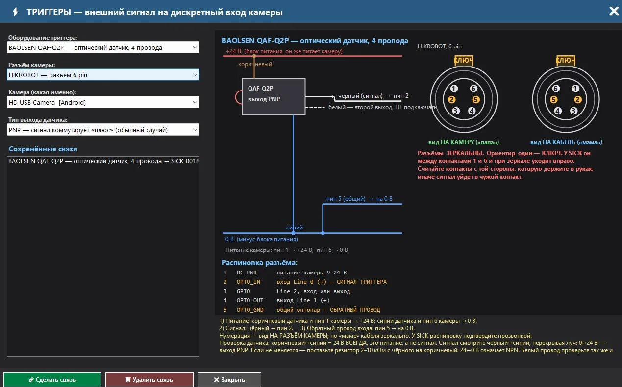
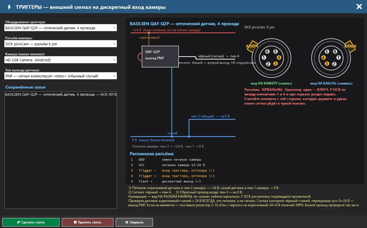
Identifying and labeling the connectors
| Pin | HIKROBOT MV-CS, 6 pin | SICK picoCam, 6 pin |
|---|---|---|
| 1 | DC_PWR – Camera power supply: 9–24 V | GND — camera power supply ground |
| 2 | OPTO_IN — Line 0 input (+), trigger signal | VCC — camera power supply (12–24V) |
| 3 | GPIO — Line 2, input or output | Trigger input – optocoupler (−) |
| 4 | OPTO_OUT — Output of Line 1 (+) | Trigger + – Trigger input, phototransistor (+) |
| 5 | OPTO_GND — a common optical fiber, with a return path | Flash + — discrete output (+) |
| 6 | GND — camera power supply ground | Flash − — discrete output (-) |
7. Outputs: rejector, camera discrete outputs, and TCP
The rejector converts the inspection result into an action. The rule is created for a specific area (or for all areas of the model, class, or marked areas) and is triggered when the model detects the specified class in that area. The actions are three: sending a TCP packet to the robot or PLC, switching the camera's digital output, and issuing an audible alert to the operator. Each trigger is recorded in the log.
7.1. OUTPUT REFERENCE: Contacts and testing with a multimeter
The "EXIT" button on the video opens a help window that does not configure anything: it shows which contacts are used for the output, how to test it without power, and how to connect a load.
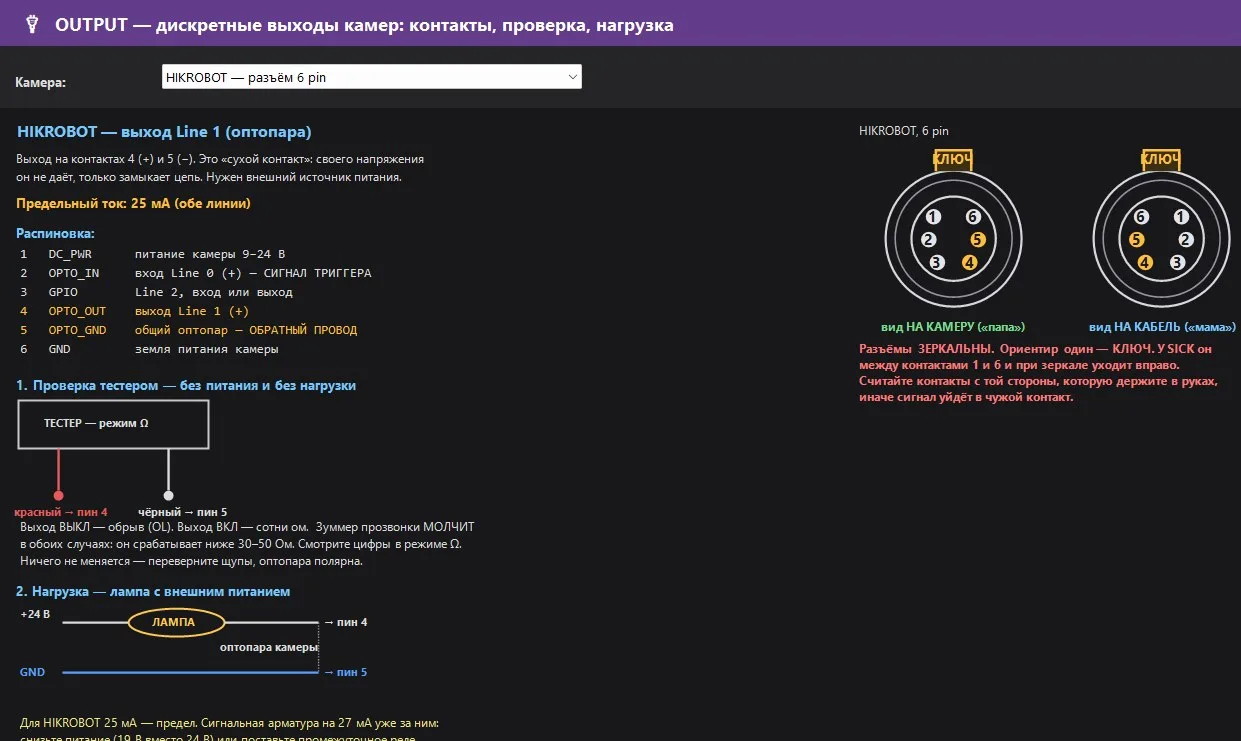
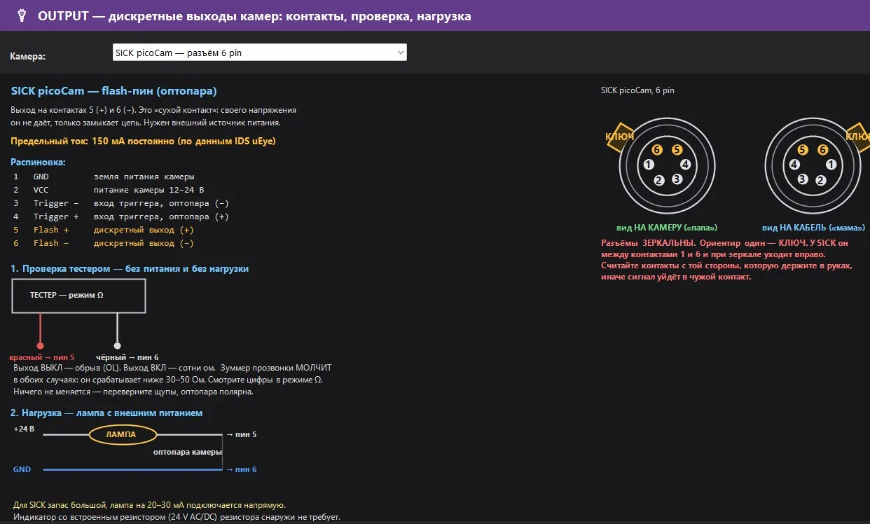
- Output — "dry contact" of the photo-relay: it does not provide its own voltage, only closes the circuit. An external power supply is required.
- Testing with a multimeter in Ω mode: OUTPUT OFF — open circuit (OL), OUTPUT ON — hundreds of Ohms. The buzzer is silent in both cases, see the numbers. If nothing changes, reverse the probes; the photo-relay is polarized.
- Load: +24V → lamp → pin "+", pin "-" → GND. For HIKROBOT, the limit is 25mA – any signal exceeding 27mA will cause problems; reduce the power supply or use an intermediate relay. For SICK, the power consumption is high, typically 20-30mA per lamp, which can be connected directly.
7.2. OUTPUT Window: Zone Rule
The "OUTPUT" button on the right panel (or right-clicking on the area → "Create a rejector for this area") opens the "OUTPUT – TCP packets and camera discrete outputs" window. On the left, there is a tree structure "Cameras → AI models → classes → zones" with checkboxes on the zones; on the right, there are tabs for "Zone rules", "Trigger log", and "Database".
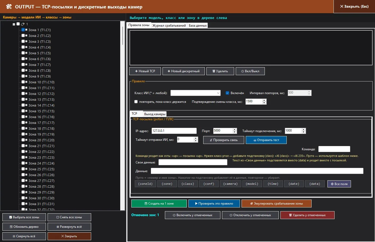
One zone can contain multiple TCP rules (different receivers), no more than one discrete output rule per class, and no more than one audio stream per class. The rule is stored in the database and operates from the inference stream: rules are stored in memory, a search for the zone's address is performed per frame, and the camera's sockets and SDK are handled by a separate dispatcher thread to prevent the analysis from waiting for the network.
7.3. TCP Packet to Robot or PLC
The program functions as a TCP client: it connects to the specified IP address and port of the receiver, maintains the connection, and reuses it. If the connection is lost, it attempts to reconnect and resend the data once. The data is transmitted in UTF-8 encoding and includes a carriage return and line feed character at the end.
| Field | Purpose |
|---|---|
| Connection timeout, ms | Default: 1000, 100…10000. |
| AI sending timeout, ms | Minimum pause between automatic rule transmissions; 0 = no pause. Even changing the class requires this pause. |
| Command | The word is transcribed exactly: "up" – the "up" package. A class angle is needed – add a placeholder: "J6 {class}" → "J6 235". Empty – uses the "Data" template. |
| Own data | Placeholder text that can be inserted in place of `{data}`. |
| Data | Template for a package. Empty = "zone number and name" ({zoneId} {zone}). Clicking on the placeholder adds it; clicking again removes it; "All fields" creates a structured template. |
| Substitution | Meaning | Substitution | Meaning |
|---|---|---|---|
| {zoneId} | Zone number (1, 2, 3…) | {camera} | Camera name |
| {zone} | Zone name (editable in the database) | {model} | AI model name |
| {class} | Class the model identified | {time} | Time HH:MM:SS.ms |
| {conf} | Confidence, % (using a dot as a decimal separator) | {date} | Date YYYY-MM-DD |
| {data} | Text from "Own Data" |
Example of a structured template: zoneId={zoneId};zone={zone};class={class};conf={conf};camera={camera};model={model};time={time};date={date};data={data}. Numbers are always in a consistent format to prevent parsing errors in PLCs.
- `Check connection` only opens the socket and reports either "connection established" or "no response after N ms".
- Send Test actually sends a string; the result is displayed next to the button, not within the window.
- Confirmation. Without the "repeat" checkbox, the rule sends one message upon class change and repeats it until the recipient responds with the line ok <message>. With the checkbox, the message is repeated at regular intervals while the class remains active.
- "Last command wins": If the model has generated multiple results while the operator is busy, the last one will be executed. The queue is limited to 512 tasks.
7.4. Discrete Camera Output
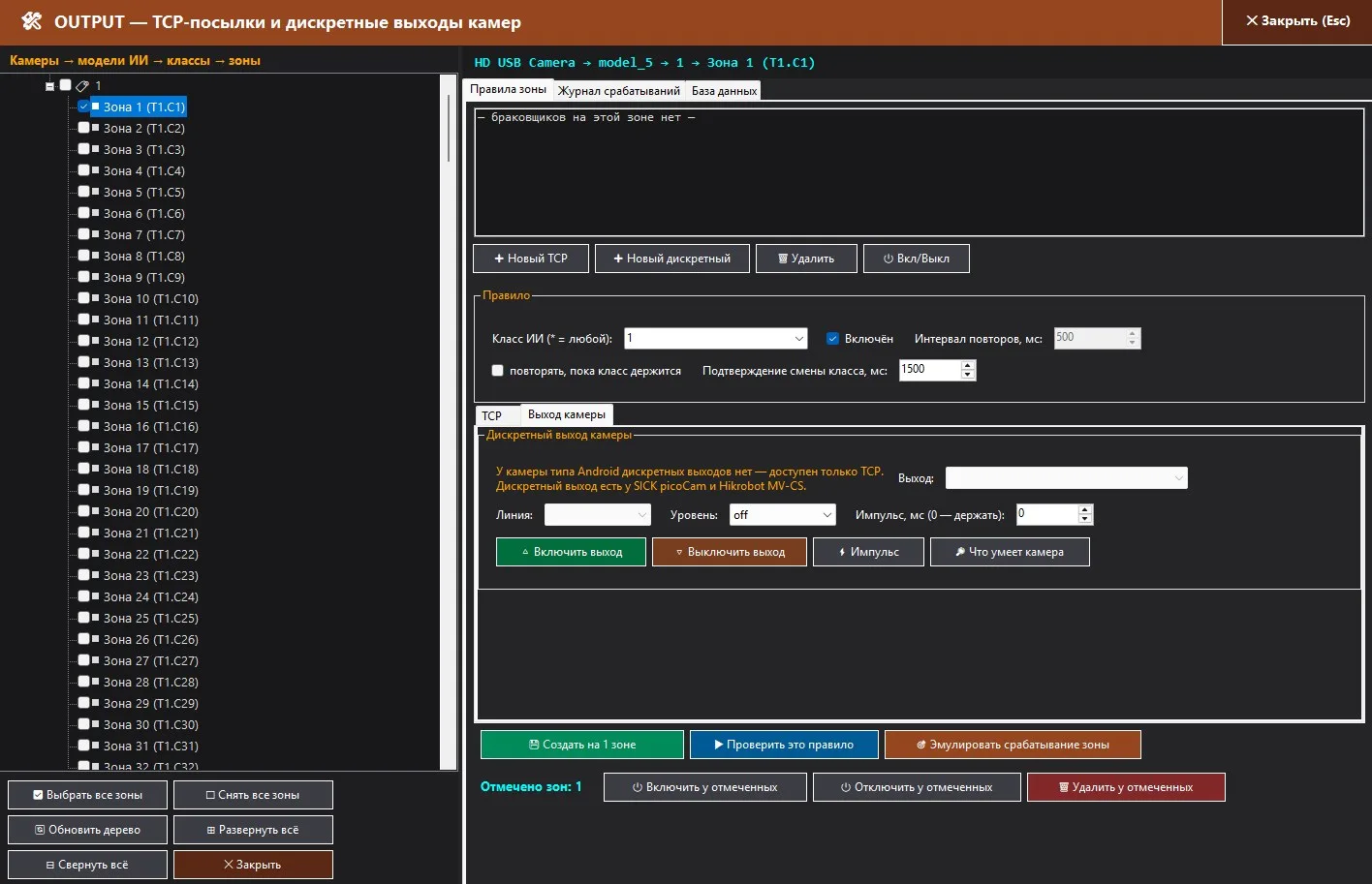
| Field | Purpose |
|---|---|
| Output | Method: Auto (SICK – Flash pin (constant level) or GPIO; HIKROBOT – UserOutputValue or LineInverter (strobing off)). The MV-CS020/016-10GC UserOutput node does not have a UserOutput – the program will automatically select LineInverter. |
| Line | Flash pin / GPIO1…6 (SICK); Line1 (output), Line2 (bidirectional) (HIKROBOT); Line0 – only input. |
| Level | true / false / off. "off" – rule is active, but the output is not affected. |
| Pulse, ms (0 – hold) | 0 – level is held until the class changes; otherwise, a pulse of 10…5000 ms with return. |
The buttons Enable Output, Disable Output, and Pulse are checked using a tester or lamp; What the camera can do queries all methods and prints a report. Manual tests are written in the same log.
7.5. Audio Alert: Custom sound for each zone
The third type of rule involves audio alerts from the computer running the software. The operator doesn't need to look at the screen; instead, they hear an alert when a zone enters a defective state, and different sounds in different zones indicate the specific location. This audio alert is available for any cameras, including USB and RTSP cameras, which do not have discrete outputs.
| Behavior | How it works |
|---|---|
| Without the "repeat" checkbox. | The sound occurs once after a confirmed change in zone class (after "Zone Class Change Confirmation"). As long as the class remains unchanged, there is silence. |
| With the "repeat until the class is still" checkbox. | The signal repeats according to the "Repetition Interval," but not more frequently than the pause between sounds, as long as the area remains within the specified class. |
| Several areas in the defect simultaneously | Each zone produces its own sound; signals from different zones do not interfere with each other, but only the signal from a single zone is silenced. |
| Journal | Each trigger is recorded in the "Trigger Log" as a line stating "Sound: …"; if the file is not found or the audio device fails, the line indicates an error, and the program continues to function. |
| Verification | Verify this rule immediately plays the sound; Simulate zone activation plays the sound along with TCP and outputs through the combat queue. |
7.6. Trigger Log and Database
The "Operation Log" tab displays the most recent 300 entries in rows of the format "HH:MM:SS.mmm ✔/✖ Camera · Model · Class · Zone → Action [message]", and it is updated in real-time. The "Refresh" and "Clear Log" buttons.
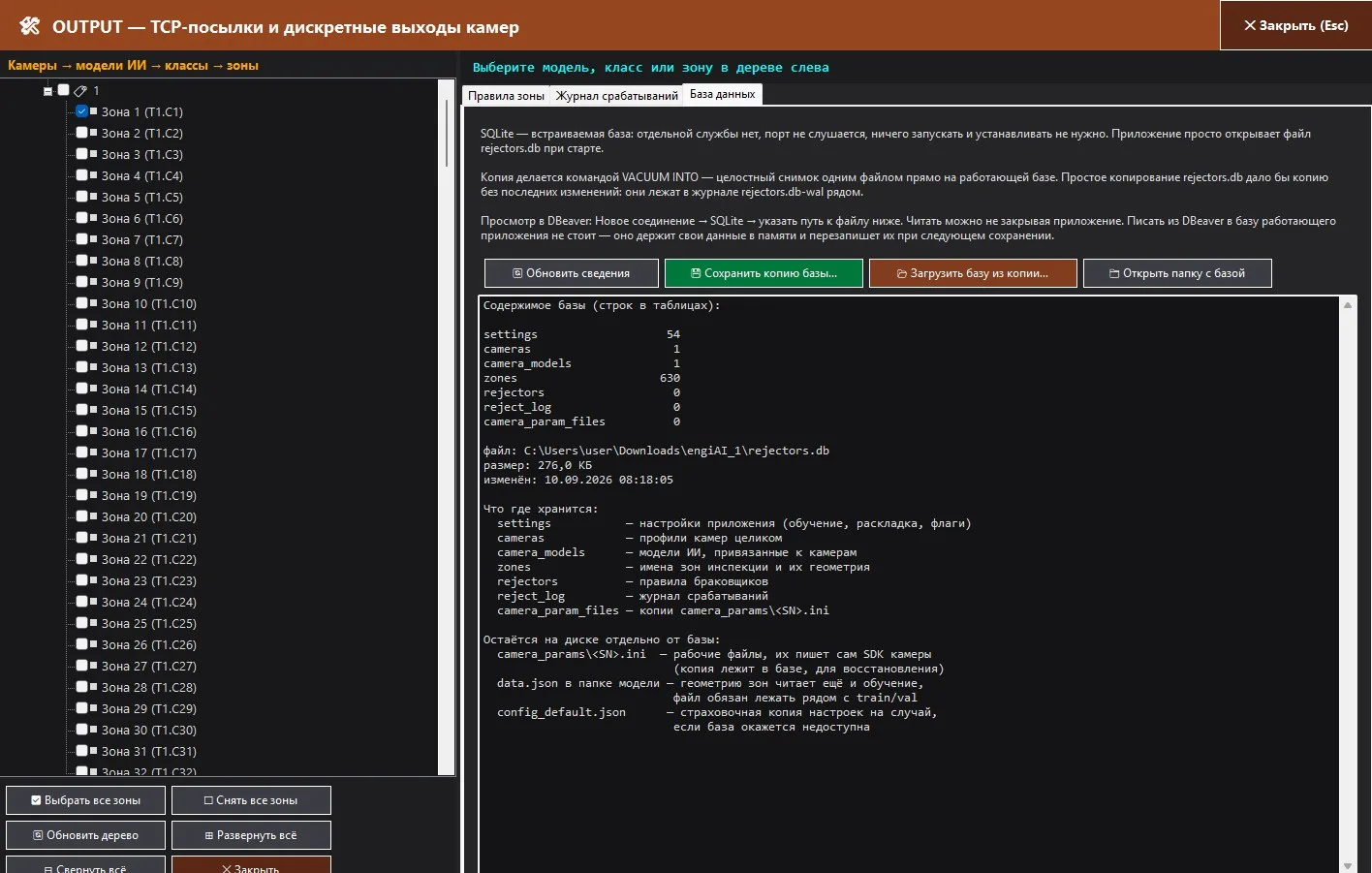
Tab DatabaseThe program stores all data in a SQLite file rejectors.db Next to the executable file, there is no separate service running, and the port is not active. No installation is required. Tables: "settings" (settings), "cameras" (camera profiles) camera_models (models on cameras), zones (zone names and geometry), rejectors (rules) reject_log (journal) camera_param_files (copies of camera settings), camera_presets (camera settings configurations). Save a copy of the database... It creates a comprehensive snapshot of the VACUUM INTO process directly on the active database. Load the database from a copy... It restores the database, but first saves the current version. You can view the database in DBeaver without closing the program; however, you should avoid modifying it from outside the program.
8. Other Modes and Tasks
Standard models: normal / anomaly and any classes
The same ROI editor also works for standard classification: pills, caps, labels, and parts in the tray. The classes are defined in the "New AI Model" dialogue (default: normal and anomaly, with Latin characters), and the zones are assigned to the items. The "Take a picture" button with numbers 1…50, the "Create images" series, either from the camera (frame/shot) or from the encoder, and the "Synthetic data for AI" panel: precise rotations of 90°/180°, a full 360° rotation with a step and range, a mirror, "classes by degrees" (each angle in its own class – the rejector sends the angle via TCP), and brightness and contrast ranges. Training is performed with full Ultralytics augmentations. The confidence threshold for these models is set in the same place as for ZONE-PAIR – on the Inspect tab.
Multi-model inspection (slots 1–20)
With a single camera, you can manage up to 20 models: Add ONNX to the slot, then ROI → Add a class to the selected model – each model in the slot has its own zone labeling, and the results from all models are displayed on a single frame.
When multi-model inspection is actually used:
| Situation | How to configure |
|---|---|
| Different tasks on a single frame | ZONE-PAIR checks the layout and the presence of elements, while the standard model in the second slot marks the item with a label, sticker, color, or key direction. The zones of the second model are added separately using "ROI → Add class to selected model". |
| Product without a fixed grid | Tablets, covers, and components in the tray: multiple product types in standard models. Similar types are arranged in different slots to prevent confusion. |
| Two different boards in one frame | Two ZONE-PAIR models in different slots, each with its own reference and grid. The live conveyor works with the reference of the main model. |
| Transition period | The old, trained model remains in the slot while the new ZONE-PAIR gathers statistics; both are visible on the same frame, and the rejector rules are transferred as trust increases. |
The threshold, analysis speed, yellow zones, and rejector rules apply to all camera models. The "REMOVE MODEL" button clears and resets the slots, so it asks for confirmation; "Remove selected" removes one model from the slot, but its files and zones remain in the database.
Common models
The "GENERAL MODELS" button saves a set of "camera → model" entries under the name: "Create from current models", "Apply to all cameras", "Update from current", "Rename", "Delete set". Switching the stand from eight cameras to another product is a single selection. Deleting the set only removes the grouping: folders, ONNX, zones, and rules remain. The zones belong to the pair "camera + model": one model on eight cameras results in eight independent annotations.
Encoder and rejector on the conveyor
For lines with an encoder on the COM port (115200, ESP32): connect CONNECT ENCODER, auto-connect, position, image capture step, and correction, Set zero + CAPTURE. Capture for training and analysis can be done "via the encoder" - the frames are evenly spaced along the product's path. The old rejector, with a time delay and anti-spam function, sends the REJECT command to the encoder controller.
Video and image recording
Settings tab: START VIDEO RECORDING from the active camera to a file named record_date_time.avi (MJPG, actual camera FPS). Training images: real_….jpg, inspection images: inspect_….jpg with marked areas.
9. Settings, console, requirements, and license
Settings
- SAVE TO FILE / LOAD FROM FILE – all settings (camera, models, rules) in JSON format, which is convenient before reinstalling or transferring to a second computer. The source of truth is the database, and the JSON file serves as a backup in case the database becomes unavailable. All changes to the settings are automatically saved.
- RESET TO DEFAULT – This action is irreversible: it removes the configuration and window layout.
- Interface language: 14 languages; the main window switches immediately, and the other windows switch upon the next opening.
- Position, size, and monitor of all windows, and the position of dividers – are stored in the database; when the monitor is turned off, the window returns to the visible area.
Console
The "Camera" and "Trigger" checkboxes are disabled by default, and the corresponding messages are displayed (in trigger mode, camera messages go to the "Trigger" section); all data is written to the logs\engiai-*.log files before any filtering is applied. The console is designed to operate for weeks without intervention: up to 800 lines are displayed on the screen, with 1000 old lines being removed; new lines are collected in batches of 4 every second, rather than one at a time; downward scrolling is enabled until you manually scroll upwards; the console has no sound. Changes to zone classes are written no more than 10 lines per second (the rest is stored in a counter), the log file is 20 MB in size, and files older than 14 days are deleted upon startup; the log of events in the database stores the last 20,000 entries. Unprocessed errors are located in crash.log, and the reasons for forced termination are located in runtime.log next to the exe file. If something is not working correctly, check this section first.
Requirements
| Component | Requirement |
|---|---|
| Operating System | Windows 10/11 x64. |
| Inspection Video Card | NVIDIA with CUDA driver; CUDA 13 and cuDNN 9 libraries are included with the software. Inspection runs on the processor automatically without a video card. |
| Training | Python 3 (with the "Add python.exe to PATH" option during installation) and the ultralytics, onnx, onnxslim, onnxruntime packages – the program automatically installs them during the initial training process, requiring an internet connection. The GPU used for training is determined by PyTorch; without CUDA, training will proceed on the CPU, but at a slower pace, with the same result. |
| SICK Cameras | IDS uEye driver; the camera must be visible in IDS Camera Manager. |
| HIKROBOT Cameras | MVS SDK (library included with the software); for GigE, a network card with jumbo frame support is required. |
License and Trial Mode
Upon startup, the program connects to the engi.live license server. Only hashes of the hardware identifiers and version numbers are sent, without serial numbers or user names. If the server is unavailable, but a license has been cached, the program operates using the cached license (for offline environments). Without a valid license, a 20-minute trial mode is activated: a "TEST MM:SS" countdown appears in the window title bar and in the AI status bar. The "BUY" button on the Settings tab opens the purchase page. When a valid license is active, the countdown is not displayed.
10. Quick Checklist and Fault Finding
Zero-based checklist for the board
If something goes wrong:
| Symptom | What to check |
|---|---|
| Camera does not appear in the list | Power and cable; for SICK — IDS Camera Manager and IP from the adapter's subnet; for HIKROBOT, wait up to 25 seconds after an emergency shutdown and "Reconnect" |
| Image is dark, gray, or has incorrect colors | Camera → "Auto-configuration for AI"; for color SICK — Bayer pattern and white balance; for USB — "Standard", then "Lock parameters" |
| Frames are dropping, network is red | GigE: packet size of 1500 or jumbo on the network card, inter-packet delay; lower FPS or fewer frames; separate network card for the camera |
| "Component not found" / image missed | reference not detected or captured under different lighting; few reference points – enlarge the alignment region with details; the area contains a table or conveyor; increase the search period |
| Zones are shifting to another board | the board is searched by the inspection zones: re-establish the reference with the alignment region around the board (section 4.4); automatic alignment model |
| Defective boards from a different batch are missing | marking on the enclosures is different: add normal images from this batch; do not create synthetic scratches thinner than 3 px (section 4.6); check that the defect is a shift, not a color |
| Areas marked with NO_ZONE_CLASS | the grid changed after training; return the grid or create a new model and reshoot |
| All zones are red on a good board | another payment or different position without a live conveyor; the threshold is too high; the photos were taken under different lighting; mixed color and grayscale files |
| The model does not detect any movement of the element. | recalculate px/mm (section 1.3): with a small scale, the shift should be less than 5 px; reduce the field of view or use a camera with higher resolution; do not increase the shift |
| Learning is declining or progressing very slowly. | Device = CPU if no NVIDIA graphics card is present; reduce Batch Size; enable Console output; verify that Python is in the PATH. |
| The inspection system is not functioning correctly. | Is best.onnx selected? Is the speed source enabled (via camera / timer / trigger)? Is the "DO NOT USE AI" option unchecked? Is the "AI Enabled" checkbox selected on the camera? |
| The "rejector" rule is silent. | "Create on N zones" checkbox: checked; rule class matches the model's answer (anomaly / normal); for exit, the level is not "off"; USB cameras have no outputs, only TCP. |
| The sound isn't working. | The rule has been created and enabled; the file is located in the "sounds" (or "sounds\custom") folder; is there a pause between the sounds; when "repeat" is disabled, the sound only plays when the class changes; Windows volume and output device. |
| The TCP packet is sent only once. | The "repeat" function requires a response of "ok <package>" from the receiver; either check the "repeat while class is active" box or configure the response on the PLC side. |
engiAI Ethernet System. The names of buttons and fields are as they appear in the program on your language (screenshots are from the Russian interface). The screenshots were taken on the "model_4" model (two 256x256 zones: capacitor C30 and bridge BR1), a 3264x2448 USB camera, and the model was trained in grayscale. Version 3, September 2026: example with two zones, creating model folders, alignment region, synthetic data "element with base" with "before / after" images, color palette and line thickness, red zones, console.